9 Data aggregation

Data aggregation refers to summarizing data with statistics such as sum, count, average, maximum, minimum, etc. to provide a high level view of the data. Often there are mutually exclusive groups in the data that are of interest. In such cases, we may be interested in finding these statistics separately for each group. The Pandas DataFrame method groupby() is used to split the data into groups, and then the desired function(s) are applied on each of these groups for groupwise data aggregation. However, the groupby() method is not limited to groupwise data aggregation, but can also be used for several other kinds of groupwise operations.

Groupby mechanics: (Source: https://pandas.pydata.org/docs/user_guide/groupby.html)

Group by: split-apply-combine By ‘group by’ we are referring to a process involving one or more of the following steps:

Splitting the data into groups based on some criteria.
Applying a function to each group independently.
Combining the results in a DataFrame.

Out of these, the split step is the most straightforward. In fact, in many situations we may wish to split the data set into groups and do something with those groups. In the apply step, we may wish to do one of the following:

1. Aggregation: compute a summary statistic (or statistics) for each group. Some examples:

Compute group sums or means.
Compute group sizes / counts.

2. Transformation: perform some group-specific computations and return a like-indexed object. Some examples:

Standardize data (zscore) within a group.
Filling NAs within groups with a value derived from each group.

3. Filtration: discard some groups, according to a group-wise computation that evaluates True or False. Some examples:

Discard data that belongs to groups with only a few members.
Filter out data based on the group sum or mean.

Some combination of the above: GroupBy will examine the results of the apply step and try to return a sensibly combined result if it doesn’t fit into either of the above two categories.

We’ll use Pandas to group the data and perform GroupBy operations.

import pandas as pd
import numpy as np
import seaborn as sns
import matplotlib.pyplot as plt

9.1 The GroupBy object

9.1.1 Creating a GroupBy object: `groupby`

This Pandas DataFrame method groupby() is used to create a GroupBy object.

A string passed to groupby() may refer to either a column or an index level. If a string matches both a column name and an index level name, a ValueError will be raised.

Example: Consider the life expectancy dataset, gdp_lifeExpectancy.csv. Suppose we want to group by the observations by continent.

gdp_lifeExp_data = pd.read_csv('./Datasets/gdp_lifeExpectancy.csv')
gdp_lifeExp_data.head()

	country	continent	year	lifeExp	pop	gdpPercap
0	Afghanistan	Asia	1952	28.801	8425333	779.445314
1	Afghanistan	Asia	1957	30.332	9240934	820.853030
2	Afghanistan	Asia	1962	31.997	10267083	853.100710
3	Afghanistan	Asia	1967	34.020	11537966	836.197138
4	Afghanistan	Asia	1972	36.088	13079460	739.981106

We will pass the column continent as an argument to the groupby() method.

#Creating a GroupBy object
grouped = gdp_lifeExp_data.groupby('continent')
#This will split the data into groups that correspond to values of the column 'continent'

The groupby() method returns a GroupBy object.

#A 'GroupBy' objects is created with the `groupby()` function
type(grouped)

pandas.core.groupby.generic.DataFrameGroupBy

The GroupBy object grouped contains the information of the groups in which the data is distributed. Each observation has been assigned to a specific group of the column(s) used to group the data. However, note that the dataset is not physically split into different DataFrames. For example, in the above case, each observation is assigned to a particular group depending on the value of the continent for that observation. However, all the observations are still in the same DataFrame data.

9.1.2 Attributes and methods of the GroupBy object

9.1.2.1 `keys`

The object(s) grouping the data are called key(s). Here continent is the group key. The keys of the GroupBy object can be seen using Its keys attribute.

#Key(s) of the GroupBy object
grouped.keys

'continent'

9.1.2.2 `ngroups`

The number of groups in which the data is distributed based on the keys can be seen with the ngroups attribute.

#The number of groups based on the key(s)
grouped.ngroups

9.1.2.3 `groups`

The groups attribute of the GroupBy object contains the group labels (or names) and the row labels of the observations in each group, as a dictionary.

#The groups (in the dictionary format)
grouped.groups

{'Africa': [24, 25, 26, 27, 28, 29, 30, 31, 32, 33, 34, 35, 36, 37, 38, 39, 40, 41, 42, 43, 44, 45, 46, 47, 120, 121, 122, 123, 124, 125, 126, 127, 128, 129, 130, 131, 156, 157, 158, 159, 160, 161, 162, 163, 164, 165, 166, 167, 192, 193, 194, 195, 196, 197, 198, 199, 200, 201, 202, 203, 204, 205, 206, 207, 208, 209, 210, 211, 212, 213, 214, 215, 228, 229, 230, 231, 232, 233, 234, 235, 236, 237, 238, 239, 252, 253, 254, 255, 256, 257, 258, 259, 260, 261, 262, 263, 264, 265, 266, 267, ...], 'Americas': [48, 49, 50, 51, 52, 53, 54, 55, 56, 57, 58, 59, 132, 133, 134, 135, 136, 137, 138, 139, 140, 141, 142, 143, 168, 169, 170, 171, 172, 173, 174, 175, 176, 177, 178, 179, 240, 241, 242, 243, 244, 245, 246, 247, 248, 249, 250, 251, 276, 277, 278, 279, 280, 281, 282, 283, 284, 285, 286, 287, 300, 301, 302, 303, 304, 305, 306, 307, 308, 309, 310, 311, 348, 349, 350, 351, 352, 353, 354, 355, 356, 357, 358, 359, 384, 385, 386, 387, 388, 389, 390, 391, 392, 393, 394, 395, 432, 433, 434, 435, ...], 'Asia': [0, 1, 2, 3, 4, 5, 6, 7, 8, 9, 10, 11, 84, 85, 86, 87, 88, 89, 90, 91, 92, 93, 94, 95, 96, 97, 98, 99, 100, 101, 102, 103, 104, 105, 106, 107, 216, 217, 218, 219, 220, 221, 222, 223, 224, 225, 226, 227, 288, 289, 290, 291, 292, 293, 294, 295, 296, 297, 298, 299, 660, 661, 662, 663, 664, 665, 666, 667, 668, 669, 670, 671, 696, 697, 698, 699, 700, 701, 702, 703, 704, 705, 706, 707, 708, 709, 710, 711, 712, 713, 714, 715, 716, 717, 718, 719, 720, 721, 722, 723, ...], 'Europe': [12, 13, 14, 15, 16, 17, 18, 19, 20, 21, 22, 23, 72, 73, 74, 75, 76, 77, 78, 79, 80, 81, 82, 83, 108, 109, 110, 111, 112, 113, 114, 115, 116, 117, 118, 119, 144, 145, 146, 147, 148, 149, 150, 151, 152, 153, 154, 155, 180, 181, 182, 183, 184, 185, 186, 187, 188, 189, 190, 191, 372, 373, 374, 375, 376, 377, 378, 379, 380, 381, 382, 383, 396, 397, 398, 399, 400, 401, 402, 403, 404, 405, 406, 407, 408, 409, 410, 411, 412, 413, 414, 415, 416, 417, 418, 419, 516, 517, 518, 519, ...], 'Oceania': [60, 61, 62, 63, 64, 65, 66, 67, 68, 69, 70, 71, 1092, 1093, 1094, 1095, 1096, 1097, 1098, 1099, 1100, 1101, 1102, 1103]}

The group names are the keys of the dictionary, while the row labels are the corresponding values

#Group names
grouped.groups.keys()

dict_keys(['Africa', 'Americas', 'Asia', 'Europe', 'Oceania'])

#Group values are the row labels corresponding to a particular group
grouped.groups.values()

dict_values([Int64Index([  24,   25,   26,   27,   28,   29,   30,   31,   32,   33,
            ...
            1694, 1695, 1696, 1697, 1698, 1699, 1700, 1701, 1702, 1703],
           dtype='int64', length=624), Int64Index([  48,   49,   50,   51,   52,   53,   54,   55,   56,   57,
            ...
            1634, 1635, 1636, 1637, 1638, 1639, 1640, 1641, 1642, 1643],
           dtype='int64', length=300), Int64Index([   0,    1,    2,    3,    4,    5,    6,    7,    8,    9,
            ...
            1670, 1671, 1672, 1673, 1674, 1675, 1676, 1677, 1678, 1679],
           dtype='int64', length=396), Int64Index([  12,   13,   14,   15,   16,   17,   18,   19,   20,   21,
            ...
            1598, 1599, 1600, 1601, 1602, 1603, 1604, 1605, 1606, 1607],
           dtype='int64', length=360), Int64Index([  60,   61,   62,   63,   64,   65,   66,   67,   68,   69,   70,
              71, 1092, 1093, 1094, 1095, 1096, 1097, 1098, 1099, 1100, 1101,
            1102, 1103],
           dtype='int64')])

9.1.2.4 `size()`

The size() method of the GroupBy object returns the number of observations in each group.

#Number of observations in each group
grouped.size()

continent
Africa      624
Americas    300
Asia        396
Europe      360
Oceania      24
dtype: int64

9.1.2.5 `first()`

The first non missing element of each group is returned with the first() method of the GroupBy object.

#The first element of the group can be printed using the first() method
grouped.first()

	country	year	lifeExp	pop	gdpPercap
continent
Africa	Algeria	1952	43.077	9279525	2449.008185
Americas	Argentina	1952	62.485	17876956	5911.315053
Asia	Afghanistan	1952	28.801	8425333	779.445314
Europe	Albania	1952	55.230	1282697	1601.056136
Oceania	Australia	1952	69.120	8691212	10039.595640

9.1.2.6 `get_group()`

This method returns the observations for a particular group of the GroupBy object.

#Observations for individual groups can be obtained using the get_group() function
grouped.get_group('Asia')

	country	continent	year	lifeExp	pop	gdpPercap
0	Afghanistan	Asia	1952	28.801	8425333	779.445314
1	Afghanistan	Asia	1957	30.332	9240934	820.853030
2	Afghanistan	Asia	1962	31.997	10267083	853.100710
3	Afghanistan	Asia	1967	34.020	11537966	836.197138
4	Afghanistan	Asia	1972	36.088	13079460	739.981106
...	...	...	...	...	...	...
1675	Yemen, Rep.	Asia	1987	52.922	11219340	1971.741538
1676	Yemen, Rep.	Asia	1992	55.599	13367997	1879.496673
1677	Yemen, Rep.	Asia	1997	58.020	15826497	2117.484526
1678	Yemen, Rep.	Asia	2002	60.308	18701257	2234.820827
1679	Yemen, Rep.	Asia	2007	62.698	22211743	2280.769906

396 rows × 6 columns

9.2 Data aggregation with `groupby()` methods

9.2.1 `mean()`

This method returns the mean of each group of the GroupBy object.

9.2.1.1 Grouping observations

Example: Find the mean life expectancy, population and GDP per capita for each country since 1952.

First, we’ll group the data such that all observations corresponding to a country make a unique group.

#Grouping the observations by 'country'
grouped = gdp_lifeExp_data.groupby('country')

Now, we’ll find the mean statistics for each group with the mean() method. The method will be applied on all columns of the DataFrame and all groups.

#Finding the mean stastistic of all columns of the DataFrame and all groups
grouped.mean()

	year	lifeExp	pop	gdpPercap
country
Afghanistan	1979.5	37.478833	1.582372e+07	802.674598
Albania	1979.5	68.432917	2.580249e+06	3255.366633
Algeria	1979.5	59.030167	1.987541e+07	4426.025973
Angola	1979.5	37.883500	7.309390e+06	3607.100529
Argentina	1979.5	69.060417	2.860224e+07	8955.553783
...	...	...	...	...
Vietnam	1979.5	57.479500	5.456857e+07	1017.712615
West Bank and Gaza	1979.5	60.328667	1.848606e+06	3759.996781
Yemen, Rep.	1979.5	46.780417	1.084319e+07	1569.274672
Zambia	1979.5	45.996333	6.353805e+06	1358.199409
Zimbabwe	1979.5	52.663167	7.641966e+06	635.858042

142 rows × 4 columns

Note that if we wished to retain the continent in the above dataset, we can group the data by both continent and country. If the data is to be grouped by multiple columns, we need to put them within [] brackets:

#Grouping the observations by 'continent' and 'country'
grouped = gdp_lifeExp_data.groupby(['continent','country'])

#Finding the mean stastistic of all columns of the DataFrame and all groups
grouped.mean()

		year	lifeExp	pop	gdpPercap
continent	country
Africa	Algeria	1979.5	59.030167	1.987541e+07	4426.025973
	Angola	1979.5	37.883500	7.309390e+06	3607.100529
	Benin	1979.5	48.779917	4.017497e+06	1155.395107
	Botswana	1979.5	54.597500	9.711862e+05	5031.503557
	Burkina Faso	1979.5	44.694000	7.548677e+06	843.990665
...	...	...	...	...	...
Europe	Switzerland	1979.5	75.565083	6.384293e+06	27074.334405
	Turkey	1979.5	59.696417	4.590901e+07	4469.453380
	United Kingdom	1979.5	73.922583	5.608780e+07	19380.472986
Oceania	Australia	1979.5	74.662917	1.464931e+07	19980.595634
Oceania	New Zealand	1979.5	73.989500	3.100032e+06	17262.622813

142 rows × 4 columns

Here the data has been aggregated according to the group keys - continent and country, and a new DataFrame is created that is indexed by the unique values of continent-country.

For large datasets, it may be desirable to aggregate only a few columns. For example, if we wish to compute the means of only lifeExp and gdpPercap, then we can filter those columns in the GroupBy object (just like we filter columns in a DataFrame), and then apply the mean() method:

grouped[['lifeExp','gdpPercap']].mean()

		lifeExp	gdpPercap
continent	country
Africa	Algeria	59.030167	4426.025973
	Angola	37.883500	3607.100529
	Benin	48.779917	1155.395107
	Botswana	54.597500	5031.503557
	Burkina Faso	44.694000	843.990665
...	...	...	...
Europe	Switzerland	75.565083	27074.334405
	Turkey	59.696417	4469.453380
	United Kingdom	73.922583	19380.472986
Oceania	Australia	74.662917	19980.595634
Oceania	New Zealand	73.989500	17262.622813

142 rows × 2 columns

9.2.1.2 Grouping columns

By default, the grouping takes place by rows. However, as with several other Pandas methods, grouping can also be done by columns by using the axis = 1 argument.

Example: Consider we have the above dataset in the wide-format as follows.

gdp_lifeExp_data_wide = gdp_lifeExp_data.pivot(index = ['continent','country'],columns = 'year')
gdp_lifeExp_data_wide

		lifeExp										...	gdpPercap
	year	1952	1957	1962	1967	1972	1977	1982	1987	1992	1997	...	1962	1967	1972	1977	1982	1987	1992	1997	2002	2007
continent	country
Africa	Algeria	43.077	45.685	48.303	51.407	54.518	58.014	61.368	65.799	67.744	69.152	...	2550.816880	3246.991771	4182.663766	4910.416756	5745.160213	5681.358539	5023.216647	4797.295051	5288.040382	6223.367465
	Angola	30.015	31.999	34.000	35.985	37.928	39.483	39.942	39.906	40.647	40.963	...	4269.276742	5522.776375	5473.288005	3008.647355	2756.953672	2430.208311	2627.845685	2277.140884	2773.287312	4797.231267
	Benin	38.223	40.358	42.618	44.885	47.014	49.190	50.904	52.337	53.919	54.777	...	949.499064	1035.831411	1085.796879	1029.161251	1277.897616	1225.856010	1191.207681	1232.975292	1372.877931	1441.284873
	Botswana	47.622	49.618	51.520	53.298	56.024	59.319	61.484	63.622	62.745	52.556	...	983.653976	1214.709294	2263.611114	3214.857818	4551.142150	6205.883850	7954.111645	8647.142313	11003.605080	12569.851770
	Burkina Faso	31.975	34.906	37.814	40.697	43.591	46.137	48.122	49.557	50.260	50.324	...	722.512021	794.826560	854.735976	743.387037	807.198586	912.063142	931.752773	946.294962	1037.645221	1217.032994
...	...	...	...	...	...	...	...	...	...	...	...	...	...	...	...	...	...	...	...	...	...	...
Europe	Switzerland	69.620	70.560	71.320	72.770	73.780	75.390	76.210	77.410	78.030	79.370	...	20431.092700	22966.144320	27195.113040	26982.290520	28397.715120	30281.704590	31871.530300	32135.323010	34480.957710	37506.419070
	Turkey	43.585	48.079	52.098	54.336	57.005	59.507	61.036	63.108	66.146	68.835	...	2322.869908	2826.356387	3450.696380	4269.122326	4241.356344	5089.043686	5678.348271	6601.429915	6508.085718	8458.276384
	United Kingdom	69.180	70.420	70.760	71.360	72.010	72.760	74.040	75.007	76.420	77.218	...	12477.177070	14142.850890	15895.116410	17428.748460	18232.424520	21664.787670	22705.092540	26074.531360	29478.999190	33203.261280
Oceania	Australia	69.120	70.330	70.930	71.100	71.930	73.490	74.740	76.320	77.560	78.830	...	12217.226860	14526.124650	16788.629480	18334.197510	19477.009280	21888.889030	23424.766830	26997.936570	30687.754730	34435.367440
Oceania	New Zealand	69.390	70.260	71.240	71.520	71.890	72.220	73.840	74.320	76.330	77.550	...	13175.678000	14463.918930	16046.037280	16233.717700	17632.410400	19007.191290	18363.324940	21050.413770	23189.801350	25185.009110

142 rows × 36 columns

Now, find the mean GDP per capita, life expectancy and population for each country.

Here, we can group by the outer level column labels to obtain the means. Also, we need to use the argument axis=1 to indicate that we intend to group columns, instead of rows.

gdp_lifeExp_data_wide.groupby(axis=1,level=0).mean()

		gdpPercap	lifeExp	pop
continent	country
Africa	Algeria	4426.025973	59.030167	1.987541e+07
	Angola	3607.100529	37.883500	7.309390e+06
	Benin	1155.395107	48.779917	4.017497e+06
	Botswana	5031.503557	54.597500	9.711862e+05
	Burkina Faso	843.990665	44.694000	7.548677e+06
...	...	...	...	...
Europe	Switzerland	27074.334405	75.565083	6.384293e+06
	Turkey	4469.453380	59.696417	4.590901e+07
	United Kingdom	19380.472986	73.922583	5.608780e+07
Oceania	Australia	19980.595634	74.662917	1.464931e+07
Oceania	New Zealand	17262.622813	73.989500	3.100032e+06

142 rows × 3 columns

9.2.2 Practice exercise 1

Read the table consisting of GDP per capita of countries from the webpage: https://en.wikipedia.org/wiki/List_of_countries_by_GDP_(nominal)_per_capita .

To only read the relevant table, read the tables that contain the word ‘Country’.

Estimate the GDP per capita of each country as the average of the estimates of the three agencies - IMF, United Nations and World Bank.

We need to do a bit of data cleaning before we could directly use the groupby() function. Follow the steps below to answer this question:

Set the first 2 columns containing country, and UN region as hierarchical row labels.
Apply the following function on all the columns to convert them to numeric: f = lambda x:pd.to_numeric(x,errors = 'coerce')
Now use groupby() to find estimate the GDP per capita for each country.

Solution:

dfs = pd.read_html('https://en.wikipedia.org/wiki/List_of_countries_by_GDP_(nominal)_per_capita', match = 'Country')
gdp_per_capita = dfs[0]
gdp_per_capita_reindexed = gdp_per_capita.set_index([('Country/Territory','Country/Territory'),
                                                     ('UN Region','UN Region')])
gdp_per_capita_numeric=gdp_per_capita_reindexed.apply(lambda x:pd.to_numeric(x,errors = 'coerce'))
gdp_per_capita_numeric.groupby(axis=1,level=1).mean().drop(columns='Year')

9.2.3 `agg()`

Directly applying the aggregate methods of the GroupBy object such as mean, count, etc., lets us apply only one function at a time. Also, we may wish to apply an aggregate function of our own, which is not there in the set of methods of the GroupBy object, such as the range of values of a column.

The agg() function of a GroupBy object lets us aggregate data using:

Multiple aggregation functions
Custom aggregate functions (in addition to in-built functions like mean, std, count etc.)

Consider the spotify dataset containing information about tracks and artists.

spotify_data = pd.read_csv('./Datasets/spotify_data.csv')
spotify_data.head(3)

	artist_followers	genres	artist_name	artist_popularity	track_name	duration_ms	explicit	release_year	danceability	...	key	loudness	mode	speechiness	acousticness	instrumentalness	liveness	valence	tempo	time_signature
0	16996777	rap	Juice WRLD	96	All Girls Are The Same	165820	1	2021	0.673	...	0	-7.226	1	0.306	0.0769	0.000338	0.0856	0.203	161.991	4
1	16996777	rap	Juice WRLD	96	Lucid Dreams	239836	1	2021	0.511	...	6	-7.230	0	0.200	0.3490	0.000000	0.3400	0.218	83.903	4
2	16996777	rap	Juice WRLD	96	Hear Me Calling	189977	1	2021	0.699	...	7	-3.997	0	0.106	0.3080	0.000036	0.1210	0.499	88.933	4

3 rows × 21 columns

Suppose, we wish to find the average popularity of tracks for each genre. We can do that by using the mean() method of a GroupBy object, as shown in the previous section. We will also sort the table by decreasing average popularity.

grouped=spotify_data.groupby('genres')
grouped['track_popularity'].mean().sort_values(ascending = False)

genres
rap              51.162959
hip hop          48.700665
metal            46.334539
electronic       43.253165
country          41.132686
pop              37.783194
latin            37.563765
rock             36.749623
miscellaneous    36.167401
pop & rock       35.619242
hoerspiel        31.258670
folk             29.716767
jazz             20.349472
Name: track_popularity, dtype: float64

Let us also find the standard deviation of the popularity of the tracks for each genre. We will also sort the table by decreasing standard deviation of popularity.

grouped['track_popularity'].std().sort_values(ascending = False)

genres
rap              20.912240
country          20.544338
pop              17.790385
miscellaneous    16.240129
electronic       16.075841
pop & rock       15.560975
folk             15.150717
jazz             15.087119
latin            14.492199
rock             14.350580
metal            14.331154
hip hop          12.824901
hoerspiel         6.459370
Name: track_popularity, dtype: float64

Even though rap is the most popular genre on an average, its popularity varies the most amongs listeners. So, it should probably be recommended only to rap listeners or the criteria to accept rap songs on Spotify should be more stringent.

9.2.3.1 Multiple aggregate functions

Let us use the agg() method of the GroupBy object to simultaneously find the mean and standard deviation of the track popularity for each genre.

For aggregating by multiple functions, we pass a list of strings to agg(), where the strings are the function names.

grouped['track_popularity'].agg(['mean','std']).sort_values(by = 'mean',ascending = False)

	mean	std
genres
rap	51.162959	20.912240
hip hop	48.700665	12.824901
metal	46.334539	14.331154
electronic	43.253165	16.075841
country	41.132686	20.544338
pop	37.783194	17.790385
latin	37.563765	14.492199
rock	36.749623	14.350580
miscellaneous	36.167401	16.240129
pop & rock	35.619242	15.560975
hoerspiel	31.258670	6.459370
folk	29.716767	15.150717
jazz	20.349472	15.087119

From the above table, we observe that people not just like hip-hop the second most on average, but they also like it more consistently than almost all other genres. We have also sorted the above table by decreasing average track popularity.

9.2.3.2 Custom aggregate functions

In addition to the mean and standard deviation of the track popularirty of each genre, let us also include the \(90^{th}\) percentile of track popularity in the table above, and sort it by the same.

#Defining a function that returns the 90th percentile value
def Ninety_pc(x):
    return x.quantile(0.9)

grouped['track_popularity'].agg(['mean','std',Ninety_pc]).sort_values(by = 'Ninety_pc',ascending = False)

	mean	std	Ninety_pc
genres
rap	51.162959	20.912240	74
country	41.132686	20.544338	67
hip hop	48.700665	12.824901	64
metal	46.334539	14.331154	63
electronic	43.253165	16.075841	61
pop	37.783194	17.790385	60
miscellaneous	36.167401	16.240129	57
latin	37.563765	14.492199	56
pop & rock	35.619242	15.560975	56
rock	36.749623	14.350580	56
folk	29.716767	15.150717	50
jazz	20.349472	15.087119	43
hoerspiel	31.258670	6.459370	37

From the above table, we observe that even though country songs are not as popular as hip-hop on an average, the top \(10\%\) country tracks are more popular than the top \(10\%\) hip hop tracks.

For aggregating by multiple functions & changing the column names resulting from those functions, we pass a list of tuples to agg(), where each tuple is of length two, and contains the new column name & the function to be applied.

#Simultaneous renaming of columns while grouping
grouped['track_popularity'].agg([('Average','mean'),('Standard deviation','std'),('90th percentile',Ninety_pc)]).sort_values(by = '90th percentile',ascending = False)

	Average	Standard deviation	90th percentile
genres
rap	51.162959	20.912240	74
country	41.132686	20.544338	67
hip hop	48.700665	12.824901	64
metal	46.334539	14.331154	63
electronic	43.253165	16.075841	61
pop	37.783194	17.790385	60
miscellaneous	36.167401	16.240129	57
latin	37.563765	14.492199	56
pop & rock	35.619242	15.560975	56
rock	36.749623	14.350580	56
folk	29.716767	15.150717	50
jazz	20.349472	15.087119	43
hoerspiel	31.258670	6.459370	37

We can put use a lambda function as well instead of separately defining the function Ninety_pc in the above code:

#Simultaneous renaming of columns while grouping
grouped['track_popularity'].agg([('Average','mean'),('Standard deviation','std'),('90th percentile',lambda x:x.quantile(0.9))]).sort_values(by = '90th percentile',ascending = False)

	Average	Standard deviation	90th percentile
genres
rap	51.162959	20.912240	74
country	41.132686	20.544338	67
hip hop	48.700665	12.824901	64
metal	46.334539	14.331154	63
electronic	43.253165	16.075841	61
pop	37.783194	17.790385	60
miscellaneous	36.167401	16.240129	57
latin	37.563765	14.492199	56
pop & rock	35.619242	15.560975	56
rock	36.749623	14.350580	56
folk	29.716767	15.150717	50
jazz	20.349472	15.087119	43
hoerspiel	31.258670	6.459370	37

9.2.3.3 Grouping by multiple columns

Let us find aggregate statistics when we group data by multiple columns. For that, let us create a new categorical column energy_lvl that has two levels - Low energy and High energy, depending on the energy of the track.

#Creating a new categorical column 'energy_lvl'
spotify_data['energy_lvl'] = pd.qcut(spotify_data.energy,2,labels=['Low energy', 'High energy'])

Now, let us find the mean, standard deviation and 90th percentile value of the track popularity for each genre-energy level combination simultaneously.

#Grouping the data with 'genres' and 'energy_lvl'
grouped=spotify_data.groupby(['genres','energy_lvl'])

#Finding aggregate statistics of data grouped with multple columns
grouped['track_popularity'].agg(['mean','std',Ninety_pc])

		mean	std	Ninety_pc
genres	energy_lvl
country	Low energy	34.982069	19.877274	64.0
country	High energy	49.859100	18.196092	69.0
electronic	Low energy	43.754789	13.294925	59.0
electronic	High energy	43.005671	17.290356	61.2
folk	Low energy	29.617831	15.360910	51.0
folk	High energy	29.991957	14.556622	49.0
hip hop	Low energy	50.283669	12.423124	66.0
hip hop	High energy	48.012067	12.936656	63.0
hoerspiel	Low energy	31.534779	5.953968	37.0
hoerspiel	High energy	30.514032	7.609088	38.0
jazz	Low energy	19.421085	14.599499	41.0
jazz	High energy	25.715373	16.662754	50.0
latin	Low energy	34.308370	15.126721	53.0
latin	High energy	39.992605	13.504109	58.0
metal	Low energy	38.612403	16.000151	60.4
metal	High energy	46.985621	13.993685	64.0
miscellaneous	Low energy	34.157235	16.516910	56.0
miscellaneous	High energy	39.394186	15.241620	59.0
pop	Low energy	34.722631	18.340408	59.0
pop	High energy	40.597155	16.784034	61.0
pop & rock	Low energy	32.987221	15.594202	54.0
pop & rock	High energy	37.413357	15.280915	57.0
rap	Low energy	57.177966	16.491203	75.0
rap	High energy	48.225166	22.182320	74.0
rock	Low energy	34.654871	14.387263	54.0
rock	High energy	38.256199	14.133726	57.0

For most of the genres, there is not much difference between the average popularity of low energy and high energy tracks. However, in case of country tracks people seem to to prefer high energy tracks a lot more as compared to low energy tracks.

9.2.3.4 Multiple aggregate functions on multiple columns

Let us find the mean and standard deviation of track popularity and danceability for each genre and energy level.

spotify_popularity_danceability = grouped[['track_popularity','danceability']].agg([('Average','mean'),('Standard deviation','std')])
spotify_popularity_danceability

		track_popularity		danceability
		Average	Standard deviation	Average	Standard deviation
genres	energy_lvl
country	Low energy	34.982069	19.877274	0.602382	0.128027
country	High energy	49.859100	18.196092	0.597569	0.105243
electronic	Low energy	43.754789	13.294925	0.563125	0.242978
electronic	High energy	43.005671	17.290356	0.634216	0.152565
folk	Low energy	29.617831	15.360910	0.510957	0.152062
folk	High energy	29.991957	14.556622	0.564669	0.136981
hip hop	Low energy	50.283669	12.423124	0.731064	0.134749
hip hop	High energy	48.012067	12.936656	0.714225	0.125525
hoerspiel	Low energy	31.534779	5.953968	0.673494	0.072998
hoerspiel	High energy	30.514032	7.609088	0.628369	0.083672
jazz	Low energy	19.421085	14.599499	0.503981	0.147328
jazz	High energy	25.715373	16.662754	0.599330	0.135762
latin	Low energy	34.308370	15.126721	0.559290	0.158853
latin	High energy	39.992605	13.504109	0.644309	0.137094
metal	Low energy	38.612403	16.000151	0.409464	0.146364
metal	High energy	46.985621	13.993685	0.420022	0.123839
miscellaneous	Low energy	34.157235	16.516910	0.543357	0.188526
miscellaneous	High energy	39.394186	15.241620	0.629966	0.146947
pop	Low energy	34.722631	18.340408	0.544546	0.158974
pop	High energy	40.597155	16.784034	0.628555	0.136695
pop & rock	Low energy	32.987221	15.594202	0.533666	0.150233
pop & rock	High energy	37.413357	15.280915	0.554165	0.138734
rap	Low energy	57.177966	16.491203	0.712144	0.139155
rap	High energy	48.225166	22.182320	0.729174	0.130477
rock	Low energy	34.654871	14.387263	0.533698	0.160000
rock	High energy	38.256199	14.133726	0.510587	0.149943

We get a couple of insights from the above table:

High energy songs have higher danceability for most genres as expected. However, for hip-hop, country, rock and hoerspiel, even low-energy songs have comparable danceability.
Hip hop has the highest danceability as expected. However, high energy rap also has relatively high danceability.

9.2.3.5 Distinct aggregate functions on multiple columns

For aggregating by multiple functions, we pass a list of strings to agg(), where the strings are the function names.

For aggregating by multiple functions such that a distinct set of functions is applied to each column, we pass a dictionary to agg(), where the keys are the column names on which the function is to be applied, and the values are the list of strings that are the function names, or a list of tuples if we also wish to name the aggregated columns.

Example: For each genre and energy level, find the mean and standard deviation of the track popularity, and the minimum and maximum values of loudness.

#Specifying arguments to the function as a dictionary if distinct functions are to be applied on distinct columns
grouped.agg({'track_popularity':[('Average','mean'),('Standard deviation','std')],'loudness':['min','max']})

		track_popularity		loudness
		Average	Standard deviation	min	max
genres	energy_lvl
country	Low energy	34.982069	19.877274	-23.163	-4.145
country	High energy	49.859100	18.196092	-16.763	-0.716
electronic	Low energy	43.754789	13.294925	-60.000	-4.936
electronic	High energy	43.005671	17.290356	-19.756	-0.533
folk	Low energy	29.617831	15.360910	-28.715	-0.972
folk	High energy	29.991957	14.556622	-16.383	0.501
hip hop	Low energy	50.283669	12.423124	-25.947	-1.595
hip hop	High energy	48.012067	12.936656	-18.273	0.642
hoerspiel	Low energy	31.534779	5.953968	-29.907	-4.910
hoerspiel	High energy	30.514032	7.609088	-22.046	-2.130
jazz	Low energy	19.421085	14.599499	-60.000	-2.962
jazz	High energy	25.715373	16.662754	-27.563	-1.166
latin	Low energy	34.308370	15.126721	-31.897	-2.331
latin	High energy	39.992605	13.504109	-18.357	-1.204
metal	Low energy	38.612403	16.000151	-32.032	-4.311
metal	High energy	46.985621	13.993685	-16.244	-1.275
miscellaneous	Low energy	34.157235	16.516910	-44.410	-1.409
miscellaneous	High energy	39.394186	15.241620	-37.684	1.634
pop	Low energy	34.722631	18.340408	-41.182	-0.045
pop	High energy	40.597155	16.784034	-27.575	0.330
pop & rock	Low energy	32.987221	15.594202	-60.000	-1.823
pop & rock	High energy	37.413357	15.280915	-22.234	1.107
rap	Low energy	57.177966	16.491203	-23.611	-1.218
rap	High energy	48.225166	22.182320	-15.012	0.457
rock	Low energy	34.654871	14.387263	-42.488	-1.708
rock	High energy	38.256199	14.133726	-25.291	3.744

From the above table, we observe that high energy songs are always louder than low energy songs. High energy Rock songs can be very loud.

9.3 `apply()`: Data aggregation, filtering & transformation

With the apply() method of the GroupBy object, we can perform several operations on groups, other than data aggregation.

9.3.1 Filtering data by group

Example: Find the top 3 most popular tracks of each genre in the spotify dataset.

We’ll first define a function that sorts a dataset by decreasing track popularity and returns the top 3 rows. Then, we’ll apply this function on each group using the apply() method of the GroupBy object.

#Defining the function that finds the top 3 most popular tracks from the dataset 'x'
def top_stats(x,col='track_popularity',n=3):
    return x.sort_values(by=col,ascending = False)[0:n]

#Defining the groups in the spotify data
grouped_spotify_data = spotify_data.groupby('genres')

Now we’ll use the apply() method to apply the top_stats() function on each group of the object grouped_spotify_data.

#Top 3 tracks of each genre
top3_tracks = grouped_spotify_data.apply(top_stats)
top3_tracks.head()

		artist_followers	genres	artist_name	artist_popularity	track_name	track_popularity	duration_ms	explicit	release_year	danceability	...	loudness	mode	speechiness	acousticness	instrumentalness	liveness	valence	tempo	time_signature	energy_lvl
genres
country	4047	4755356	country	Luke Combs	85	Forever After All	82	232533	0	2020	0.487	...	-5.195	1	0.0253	0.1910	0.000000	0.0933	0.456	151.964	4	High energy
	2403	1678738	country	Morgan Wallen	88	Wasted On You	81	178520	0	2021	0.505	...	-5.240	0	0.0318	0.3730	0.001070	0.1260	0.252	196.000	3	High energy
	16244	1678738	country	Morgan Wallen	88	Whiskey Glasses	81	234347	0	2018	0.614	...	-4.580	1	0.0289	0.3690	0.000002	0.1150	0.707	149.959	4	High energy
electronic	83058	7650304	electronic	Daft Punk	86	One More Time	81	320357	0	2001	0.611	...	-8.618	1	0.1330	0.0193	0.000000	0.3320	0.476	122.752	4	High energy
electronic	13068	28026432	electronic	Alan Walker	85	Faded	80	212107	0	2018	0.468	...	-5.085	1	0.0476	0.0281	0.000008	0.1100	0.159	179.642	4	High energy

5 rows × 22 columns

The top_stats() function is applied to each group, and the results are concatenated internally with the concat() function. The output therefore has a hierarchical index whose outer level indices are the group keys.

We can also use a lambda function instead of separately defining the function top_tracks():

#Top 3 tracks of each genre - using lambda function
top3_tracks = grouped_spotify_data.apply(lambda x:x.sort_values(by = 'track_popularity',ascending=False)[0:3])
top3_tracks.head()

		artist_followers	genres	artist_name	artist_popularity	track_name	track_popularity	duration_ms	explicit	release_year	danceability	...	loudness	mode	speechiness	acousticness	instrumentalness	liveness	valence	tempo	time_signature	energy_lvl
genres
country	4047	4755356	country	Luke Combs	85	Forever After All	82	232533	0	2020	0.487	...	-5.195	1	0.0253	0.1910	0.000000	0.0933	0.456	151.964	4	High energy
	2403	1678738	country	Morgan Wallen	88	Wasted On You	81	178520	0	2021	0.505	...	-5.240	0	0.0318	0.3730	0.001070	0.1260	0.252	196.000	3	High energy
	16244	1678738	country	Morgan Wallen	88	Whiskey Glasses	81	234347	0	2018	0.614	...	-4.580	1	0.0289	0.3690	0.000002	0.1150	0.707	149.959	4	High energy
electronic	83058	7650304	electronic	Daft Punk	86	One More Time	81	320357	0	2001	0.611	...	-8.618	1	0.1330	0.0193	0.000000	0.3320	0.476	122.752	4	High energy
electronic	13068	28026432	electronic	Alan Walker	85	Faded	80	212107	0	2018	0.468	...	-5.085	1	0.0476	0.0281	0.000008	0.1100	0.159	179.642	4	High energy

5 rows × 22 columns

We can also pass arguments to the top_stats() function with the apply() function.

Example: Find the most popular artist from each genre.

#Applying the 'top_stats()' function to each group of the data (based on 'genre') to find the most popular artist 
#Dropping the inner row label as it is not informative
grouped_spotify_data.apply(top_stats,col='artist_popularity',n=1)['artist_name'].droplevel(axis=0, level = 1)

genres
country               Morgan Wallen
electronic                Daft Punk
folk                       Bon Iver
hip hop                      Eminem
hoerspiel              Die drei ???
jazz             Earth, Wind & Fire
latin                        Maluma
metal                   Linkin Park
miscellaneous             Pop Smoke
pop                   Justin Bieber
pop & rock                 Maroon 5
rap                       Bad Bunny
rock                Imagine Dragons
Name: artist_name, dtype: object

9.3.2 Practice exercise 2

Filter the first 4 columns of the spotify dataset. Drop duplicate observartions in the resulting dataset using the Pandas DataFrame method drop_duplicates(). Find the top 3 most popular artists for each genre.

Solution:

spotify_data.iloc[:,0:4].drop_duplicates().groupby('genres').apply(lambda x:x.sort_values(by = 'artist_popularity', 
                                                                                          ascending = False)[0:3])

9.3.3 Transforming data by group

Recall method 3 for imputing missing values in Chapter 7. The method was to impute missing values based on correlated variables in data.

In the example shown for the method, values of GDP per capita for a few countries were missing. We imputed the missing value of GDP per capita for those countries as the average GDP per capita of the corresponding continent.

We will compare the approach we used with the approach using the groupby() & apply() methods.

Let us read the datasets and the function that makes a visualization to compare the imputed values with the actual values.

#Importing data with missing values
gdp_missing_data = pd.read_csv('./Datasets/GDP_missing_data.csv')

#Importing data with all values
gdp_complete_data = pd.read_csv('./Datasets/GDP_complete_data.csv')

#Index of rows with missing values for GDP per capita
null_ind_gdpPC = gdp_missing_data.index[gdp_missing_data.gdpPerCapita.isnull()]

#Defining a function to plot the imputed values vs actual values 
def plot_actual_vs_predicted():
    fig, ax = plt.subplots(figsize=(8, 6))
    plt.rc('xtick', labelsize=15) 
    plt.rc('ytick', labelsize=15) 
    x = gdp_complete_data.loc[null_ind_gdpPC,'gdpPerCapita']
    y = gdp_imputed_data.loc[null_ind_gdpPC,'gdpPerCapita']
    plt.scatter(x,y)
    z=np.polyfit(x,y,1)
    p=np.poly1d(z)
    plt.plot(x,x,color='orange')
    plt.xlabel('Actual GDP per capita',fontsize=20)
    plt.ylabel('Imputed GDP per capita',fontsize=20)
    ax.xaxis.set_major_formatter('${x:,.0f}')
    ax.yaxis.set_major_formatter('${x:,.0f}')
    rmse = np.sqrt(((x-y).pow(2)).mean())
    print("RMSE=",rmse)

Approach 1: Using the approach we used in Section 7.1.5.3

#Finding the mean GDP per capita of the continent
avg_gdpPerCapita = gdp_missing_data['gdpPerCapita'].groupby(gdp_missing_data['continent']).mean()

#Creating a copy of missing data to impute missing values
gdp_imputed_data = gdp_missing_data.copy()

#Replacing missing GDP per capita with the mean GDP per capita for the corresponding continent
for cont in avg_gdpPerCapita.index:
    gdp_imputed_data.loc[(gdp_imputed_data.continent==cont) & (gdp_imputed_data.gdpPerCapita.isnull()),
                     'gdpPerCapita']=avg_gdpPerCapita[cont]
plot_actual_vs_predicted()

RMSE= 25473.20645170116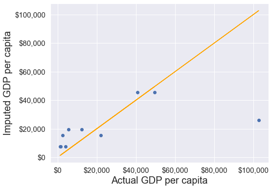

Approach 2: Using the groupby() and apply() methods.

#Creating a copy of missing data to impute missing values
gdp_imputed_data = gdp_missing_data.copy()

#Grouping data by continent
grouped = gdp_missing_data.groupby('continent')

#Applying the lambda function on the 'gdpPerCapita' column of the groups
gdp_imputed_data['gdpPerCapita'] = grouped['gdpPerCapita'].apply(lambda x: x.fillna(x.mean()))

plot_actual_vs_predicted()

RMSE= 25473.20645170116

With the apply() function, the missing value of gdpPerCapita for observations of each group are filled by the mean gdpPerCapita of that group. The code is not only more convenient to write, but also faster as compared to for loops. The for loop imputes the missing values of observations of one group at a time, while the imputation may happen in parallel for all groups with the apply() function.

9.3.4 Sampling data by group

The groupby() and apply() method can be used to for stratified random sampling from a large dataset.

The spotify dataset has more than 200k observations. It may be expensive to operate with so many observations. Suppose, we wish to take a random sample of 650 observations to analyze spotify data, such that all genres are equally represented.

Before taking the random sample, let us find the number of tracks in each genre.

spotify_data.genres.value_counts()

pop              70441
rock             49785
pop & rock       43437
miscellaneous    35848
jazz             13363
hoerspiel        12514
hip hop           7373
folk              2821
latin             2125
rap               1798
metal             1659
country           1236
electronic         790
Name: genres, dtype: int64

Let us take a random sample of 650 observations from the entire dataset.

sample_spotify_data = spotify_data.sample(650)

Now, let us see the number of track of each genre in our sample.

sample_spotify_data.genres.value_counts()

pop              185
rock             150
miscellaneous    102
pop & rock        98
jazz              37
hoerspiel         25
hip hop           22
rap                7
metal              7
latin              5
country            5
folk               5
electronic         2
Name: genres, dtype: int64

Some of the genres have a very low representation in the data. To rectify this, we can take a random sample of 50 observations from each of the 13 genres. In other words, we can take a random sample from each of the genre-based groups.

evenly_sampled_spotify_data = spotify_data.groupby('genres').apply(lambda x:x.sample(50))
evenly_sampled_spotify_data.genres.value_counts()

hoerspiel        50
hip hop          50
pop & rock       50
latin            50
country          50
rap              50
electronic       50
metal            50
folk             50
pop              50
miscellaneous    50
rock             50
jazz             50
Name: genres, dtype: int64

The above stratified random sample equally represents all the genres.

9.4 `corr()`: Correlation by group

The corr() method of the GroupBy object returns the correlation between all pairs of columns within each group.

Example: Find the correlation between danceability and track popularity for each genre-energy level combination.

spotify_data.groupby(['genres','energy_lvl']).apply(lambda x:x['danceability'].corr(x['track_popularity']))

genres         energy_lvl 
country        Low energy    -0.171830
               High energy   -0.154823
electronic     Low energy     0.378330
               High energy    0.072343
folk           Low energy     0.187482
               High energy    0.230419
hip hop        Low energy     0.113421
               High energy    0.027074
hoerspiel      Low energy    -0.053908
               High energy   -0.044211
jazz           Low energy     0.005733
               High energy    0.332356
latin          Low energy    -0.083971
               High energy    0.030276
metal          Low energy     0.127439
               High energy    0.256165
miscellaneous  Low energy     0.163185
               High energy    0.148818
pop            Low energy     0.208942
               High energy    0.156764
pop & rock     Low energy     0.063127
               High energy    0.060195
rap            Low energy    -0.008394
               High energy   -0.129873
rock           Low energy     0.027876
               High energy    0.065908
dtype: float64

The popularity of low energy electronic music is the most correlated with its danceability.

9.5 `pivot_table()`

The Pandas pivot_table() function is used to aggregate data groupwise where some of the group keys are along the rows and some along the columns. Note that pivot_table() is the same as pivot() except that pivot_table() aggregates the data as well in addition to re-arranging it.

Example: Find the mean of track popularity for each genre-energy lvl combination such that each row corresponds to a genre, and the energy levels correspond to columns.

pd.pivot_table(data = spotify_data,values = 'track_popularity',index = 'genres', columns ='energy_lvl',aggfunc = 'mean',margins = True)

energy_lvl	Low energy	High energy	All
genres
country	34.982069	49.859100	41.132686
electronic	43.754789	43.005671	43.253165
folk	29.617831	29.991957	29.716767
hip hop	50.283669	48.012067	48.700665
hoerspiel	31.534779	30.514032	31.258670
jazz	19.421085	25.715373	20.349472
latin	34.308370	39.992605	37.563765
metal	38.612403	46.985621	46.334539
miscellaneous	34.157235	39.394186	36.167401
pop	34.722631	40.597155	37.783194
pop & rock	32.987221	37.413357	35.619242
rap	57.177966	48.225166	51.162959
rock	34.654871	38.256199	36.749623
All	33.015545	39.151701	36.080772

We can use also use custom GroupBy aggregate functions with pivot_table().

Example: Find the \(90^{th}\) percentile of track popularity for each genre-energy lvl combination such that each row corresponds to a genre, and the energy levels correspond to columns.

pd.pivot_table(data = spotify_data,values = 'track_popularity',index = 'genres', columns ='energy_lvl',aggfunc = lambda x:np.percentile(x,90))

energy_lvl	Low energy	High energy
genres
country	64.0	69.0
electronic	59.0	61.2
folk	51.0	49.0
hip hop	66.0	63.0
hoerspiel	37.0	38.0
jazz	41.0	50.0
latin	53.0	58.0
metal	60.4	64.0
miscellaneous	56.0	59.0
pop	59.0	61.0
pop & rock	54.0	57.0
rap	75.0	74.0
rock	54.0	57.0

9.6 `crosstab()`

The crosstab() method is a special case of a pivot table for computing group frequncies (or size of each group). We may often use it to check if the data is representative of all groups that are of interest to us.

Example: Find the number of observations in each group, where each groups corresponds to a distinct genre-energy lvl combination

#Cross tabulation of 'genres' and 'energy_lvl'
pd.crosstab(spotify_data.genres,spotify_data.energy_lvl,margins = True).sort_values(by = 'All',ascending = False)

energy_lvl	Low energy	High energy	All
genres
All	121708	121482	243190
pop	33742	36699	70441
rock	20827	28958	49785
pop & rock	17607	25830	43437
miscellaneous	22088	13760	35848
jazz	11392	1971	13363
hoerspiel	9129	3385	12514
hip hop	2235	5138	7373
folk	2075	746	2821
latin	908	1217	2125
rap	590	1208	1798
metal	129	1530	1659
country	725	511	1236
electronic	261	529	790

The above table can be generated with the pivot_table() function using ‘count’ as the aggfunc argument, as shown below. However, the crosstab() function is more compact to code.

#Generating cross-tabulation of 'genres' and 'energy_lvl' with 'pivot_table()'
pd.pivot_table(data = spotify_data,values = 'track_popularity',index = 'genres', columns ='energy_lvl',aggfunc = 'count',margins=True)

energy_lvl	Low energy	High energy	All
genres
country	725	511	1236
electronic	261	529	790
folk	2075	746	2821
hip hop	2235	5138	7373
hoerspiel	9129	3385	12514
jazz	11392	1971	13363
latin	908	1217	2125
metal	129	1530	1659
miscellaneous	22088	13760	35848
pop	33742	36699	70441
pop & rock	17607	25830	43437
rap	590	1208	1798
rock	20827	28958	49785
All	121708	121482	243190

Example: Find the percentage of observations in each group of the above table.

pd.crosstab(spotify_data.genres,spotify_data.energy_lvl,margins = True).sort_values(by = 'All',ascending = False)/spotify_data.shape[0]*100

energy_lvl	Low energy	High energy	All
genres
All	50.046466	49.953534	100.000000
pop	13.874748	15.090670	28.965418
rock	8.564086	11.907562	20.471648
pop & rock	7.240018	10.621325	17.861343
miscellaneous	9.082610	5.658127	14.740738
jazz	4.684403	0.810477	5.494881
hoerspiel	3.753855	1.391916	5.145771
hip hop	0.919034	2.112751	3.031786
folk	0.853242	0.306756	1.159998
latin	0.373371	0.500432	0.873802
rap	0.242609	0.496731	0.739340
metal	0.053045	0.629138	0.682183
country	0.298121	0.210124	0.508245
electronic	0.107323	0.217525	0.324849

9.6.1 Practice exercise 3

What percentage of unique tracks are contributed by the top 5 artists of each genre?

Hint: Find the top 5 artists based on artist_popularity for each genre. Count the total number of unique tracks (track_name) contributed by these artists. Divide this number by the total number of unique tracks in the data. The nunique() function will be useful.

Solution:

top5artists = spotify_data.iloc[:,0:4].drop_duplicates().groupby('genres').apply(lambda x:x.sort_values(by = 'artist_popularity', 
                            ascending = False)[0:5]).droplevel(axis=0,level=1)['artist_name']
top5artists_tracks = spotify_data.loc[spotify_data.artist_name.isin(top5artists),:]
top5artists_tracks.track_name.nunique()/spotify_data.track_name.nunique()

9.1 The GroupBy object

9.1.1 Creating a GroupBy object: groupby

9.1.2 Attributes and methods of the GroupBy object

9.1.2.1 keys

9.1.2.2 ngroups

9.1.2.3 groups

9.1.2.4 size()

9.1.2.5 first()

9.1.2.6 get_group()

9.2 Data aggregation with groupby() methods

9.2.1 mean()

9.2.1.1 Grouping observations

9.2.1.2 Grouping columns

9.2.2 Practice exercise 1

9.2.3 agg()

9.2.3.1 Multiple aggregate functions

9.2.3.2 Custom aggregate functions

9.2.3.3 Grouping by multiple columns

9.2.3.4 Multiple aggregate functions on multiple columns

9.2.3.5 Distinct aggregate functions on multiple columns

9.3 apply(): Data aggregation, filtering & transformation

9.3.1 Filtering data by group

9.3.2 Practice exercise 2

9.3.3 Transforming data by group

9.3.4 Sampling data by group

9.4 corr(): Correlation by group

9.5 pivot_table()

9.6 crosstab()

9.6.1 Practice exercise 3

9.1.1 Creating a GroupBy object: `groupby`

9.1.2.1 `keys`

9.1.2.2 `ngroups`

9.1.2.3 `groups`

9.1.2.4 `size()`

9.1.2.5 `first()`

9.1.2.6 `get_group()`

9.2 Data aggregation with `groupby()` methods

9.2.1 `mean()`

9.2.3 `agg()`

9.3 `apply()`: Data aggregation, filtering & transformation

9.4 `corr()`: Correlation by group

9.5 `pivot_table()`

9.6 `crosstab()`